Reading Note:Modelling Context and Syntactical Features for Aspect-based Sentiment Analysis

From: Proceedings of the 58th Annual Meeting of the Association for Computational Linguistics
URL: https://aclanthology.org/2020.acl-main.293/
Authors: Minh Hieu Phan and Philip Ogunbona.

Something inevitable have finished recently, so I can take a rest and get ready for sharing this paper. Although it has been a while since this paper published, the main ideas of it can be valuable reference. This paper is based on two conceptual tasks of ABSA including Aspect Extraction and Aspect Sentiment Classification. In order to finish these tasks simultaneously, an end-to-end solution is built by the authors. Here are two important ideas:

• Focusing on the disadventage of previous models which ignore the syntactical information, this paper proposes the syntactic relative distance.
• To enhance the performance of Aspect Extraction, this paper ustilizes the combination of part-of-speech embeddings, dependency-based embeddings and contextualized embeddings.

Motivation

The ABSA task can be divided into two sub-tasks so it can be solved by different strategies. To some previous researches, they constructed the pipeline model to finish different sub-tasks of ABSA respectively. However, the interaction of different components in pipeline model sometimes causes the errors. Recent approaches(He et al., 2019; Wang et al., 2018; Li et al., 2019) attempted to develop the multi-tasks solutions for the task, but the core idea of them is formulating two sub-tasks as a single sequence labelling with a unified tagging scheme. Those approaches ignored the complexity of ABSA task will be raised by adding extra tokens. Also, this paper finds a problem that appears in the LCF(Local Context Focus) mechanism: the matrics of relative distance should be based on the syntactic distance, not the distance between tokens. Phan et al. proposes the following approaches and attempts to solve the above problems. And these approaches construct two models named CSAE and LCFS-ASC.

CSAE

To the proposed models, both of them ustilize the dependency tree to model the syntactic information of the sentences. Let's talk about the CSAE model first.

Figure. 1: The overall aritecture of the CSAE model

As shown in the Figure. 1, the CSAE model consists of three componments.

Dependency-based Embedding

In the Dependency-based embedding, the process starts by using a dependency tree to parse the sequence of the input words. Figure. 2 shows the result of parsing of the example.

Figure. 2: The results of parsing and the dependency relations for each word of the example

The first result of parsing is the raw result without any processing. Phan et al. considers that the complexity of the dependency relations can be simplified by removing the unnecessary prepositions. Following this idea, the result of parsing of the example becomes the second result in Figure. 2. Let's focus on the table of Figure. 2 and the second colum of the table means the relevant dependency relations of each word ("/" separates the specific dependency relation between the word and its context word; the superscript "-1" means the word is the object of the dependency relation). After getting the relevant dependency contexts of each word, the CSAE model sends them to the Dependency-based Embedding and attempts to encode the syntactical information of the sentences by self-attention mechanism.

Contextualized Embedding

To the Contextualized Embedding, the input is the sequences consist of "[CLS] + sentence + [SEP]". And after embeddings, the output is sent to the pre-trained model BERT.

POS Embedding

The part-of-speech(POS) of each word is annotated by the Universal POS tags in this paper. We denote $P= \{ p_1, p_2, ..., p_n \}$ to the POS of the input sequence. And POS Embedding transforms each POS to corresponding dense vector representation. The sequence $V^P= \{ v^p_i | i \in [1, n] \}$ contains each vector of the POS. Like the process of Denpendency-based Embedding, the output of POS Embedding is sent to the self-attention layer, too.

Finally, the CSAE model concatenates the Attended DE, BERT states and Attended POS and input them to the full connection layer. With Softmax function, the model can predict the current token is whether the aspect term.

LCFS-ASC

In this section, the second model, LCFS-ASC is introduced from scratch. Inspired by Zeng et al, 2019, this paper optimizes the Local Context Focus mechannism for Aspect Sentiment Classification. Figure. 3 illustrates the overall architecture of the model.

Figure. 3: The overall architecture of the LCFS-ASC model

Global Context and Local Context

First, Phan et al. construct the local context and global context respectively. To global context, the input format is: "[CLS] + sentence + [SEP] + aspect term + [SEP]"; To local context, the input format is more simple: "[CLS] + sentence + [SEP]". And then, local context and global context are embedded respectively, too.

Local Context Focus

To alleviate the negative influence of irrelevant tokens to the aspect, this paper applies the Context Feature Dynamic Weight/Context Feature Dynamic Mask(CDW/CDM) techniques on the local context vectors( $V^l$ ). However, differs from the previous CDW/CDM, Phan et al. propose Syntactic Relative Distance(SRD) as a new metrics for calculating the distance of different tokens. The SRD measured by the shortest distance between the corresponding nodes in the dependency-parsed tree. Figure. 4 shows the dependency parsed tree of the example.

Figure. 4: The dependency tree of the example sentence

Let's try to calculate the SRDs of different words in the example. The SRD between an aspect term "sound amplifier" and opinion word "loudly" is computed as:

$\begin{array}{c} SRD(sound, loudly) = 3, [compound \to npadvmod \to advmod] \\ \\ SRD(amplifier, loudly) = 2, [npadvmod \to advmod] \\ \\ SRD(sound \ amplifier, loudly) = average(2, 3) = 2.5 \end{array}$

After making sure the SRDs between the words of the sentence, CDW/CDM techiniques can be used.

Context Dynamic Mask The main idea of CDM is masking the less-semantic feature of the irrelevant words whose SRD to target aspect term is greater than the pre-defined threshold( $\alpha$ ). We denote the mask vector $v^m_i$ for each words of the local context, and it is computed based on the threshold $\alpha$ :

$\begin{array}{c} v^m_i = \begin{cases} O, SRD_i > \alpha \\ I, SRD_i \leq \alpha \end{cases} \\ \\ M = [v^m_1, v^m_2, ..., v^m_n] \\ \\ V^{CDM} = V^l \odot M \end{array}$

Here $O$ and $I$ are the vectors whose elements are all zero and one respectively, also both of $O$ and $I$ $\in \mathbb{R}^h$ where h is the hidden size of the contextualized embedding(and the dimension of $v^l_i$). The character $\odot$ represents the dot product of vectors and its particle effect in above equation is masking out the local context vector $V^l$ by the mask vector $M$.

Context Dynamic Weight The procedure of CDW is similar to CDM, but the difference between them is the strategy of handling less-semantic-relative context (SRD greater than the threshold). Instead of masking the less-semantic-relative context directly, CDW attempts to de-emphasizes them based on the distance to aspect terms. Here are the equation:

$\begin{array}{c} v^w_i = \begin{cases} (1 - \frac{SRD_i - \alpha}{N}) \cdot I, SRD_i > \alpha \\ I, SRD_i \leq \alpha \end{cases} \\ \\ W = [v^w_1, v^w_2, ..., v^w_n] \\ \\ V^{CDM} = V^l \odot W \end{array}$

In this equation, $N$ is the length of the sentence.

Experiment

In this section, we will talk about the detail of the experiment, including the dataset and the results of proposed models.

Dataset

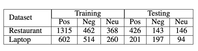
The dataset used in this paper is from SemEval2014 Task 4 Chanllenge(Pontiki et al., 2014) including the Restaurant and Laptop dataset. Table. 1 illustrates the numbers of instances in these two dataset.

Table. 1: The number of instances by polarity in Restaurant and Laptop dataset

Results

Before sharing the results of CSAE and LCFS-ASC in Restaurant and Laptop dataset, this paper compares the ability of extraction between CSAE and RoBERTa-AE(the specific model for Aspect Extraction by fine-tuning for RoBERTa). Table. 2 shows the result of such comparison.

Table. 2: The number of instances by polarity in Restaurant and Laptop dataset

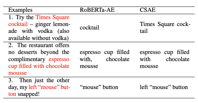
Following the result of such comparison, we can find that the RoBERTa-AE model is lack of the ability of determining the boundary of the aspect terms. However, with the information about dependency, the CSAE model can exactly extract the whole aspect terms.

Aspect Extraction

Table. 3: The result of experiment and ablation study in Aspect Extraction

Table. 3 illustrates the result of each model in Aspect Extraction task. Something interesting appears between BERT-AE and RoBERTa-AE. Although both of them are fine-tuned by the similar methods, the difference between their results is obvious. And Phan et al. considers that the reason is the pre-trained model RoBERTa removes the pre-training task which randomly masks the tokens. Also, the difference between the proposed models is worth talking about. It's no doubt that the Dependency-based Embedding and POS Embedding are helpful for Aspect Extraction task.

Aspect Sentiment Classification

Table. 4: The result of experiment and ablation study in Aspect Sentiment Classification

Table. 4 illustrates the result of each model in Aspect Sentiment Classification task. Unlike the Aspect Extraction task, the result of BERT-ASC is greater than RoBERTa-ASC, no matter the matrics is F1 score or accuracy. We can imagine the importace of random masking for Aspect Sentiment Classification. What is worth considering is the different results between LCFS-ASC-CDW and LCF-ASC-CDM. In my opinion, masking the less-semantic irrelevant words is necessary for Aspect Sentiment Classification. But the experiment demonstrates the truth that weighting those words is more appropriate.

Reference

[1] Ruidan He, Wee Sun Lee, Hwee Tou Ng, and Daniel Dahlmeier. 2019. An interactive multi-task learning network for end-to-end aspect-based sentiment analysis. arXiv preprint arXiv:1906.06906.

[2] Feixiang Wang, Man Lan, and Wenting Wang. 2018. Towards a one-stop solution to both aspect extraction and sentiment analysis tasks with neural multi-task learning. In 2018 International Joint Conference on Neural Networks (IJCNN), pages 1–8. IEEE.

[3] Xin Li, Lidong Bing, Piji Li, and Wai Lam. 2019. A unified model for opinion target extraction and target sentiment prediction. In Proceedings of the AAAI Conference on Artificial Intelligence, volume 33, pages 6714–6721.

[4] Biqing Zeng, Heng Yang, Ruyang Xu, Wu Zhou, and Xuli Han. 2019. Lcf: A local context focus mecha- nism for aspect-based sentiment classification. Applied Sciences, 9(16):3389.

[5] Maria Pontiki, Dimitris Galanis, John Pavlopoulos, Harris Papageorgiou, Ion Androutsopoulos, and Suresh Manandhar. 2014. Semeval-2014 task 4: Aspect-based sentiment analysis. In Proceedings of the 8th International Workshop on Semantic Evalua- tion (SemEval 2014), pages 27–35.